
| Version 14 (modified by , 13 years ago) (diff) |
|---|
VisIt tutorial for PRACE SoHPC at EPCC
This tutorial is a compilation of the tutorial made by Brandt Westing from the Texas Advanced Computing Center, University of Texas at Austin, and modified for newer version of VisIt 2.6.2.
Example data noise.silo is part of VisIt data samples.
To be able to run VisIt at EPCC prepare the PATH environment by typing:
export PATH=/opt/visit-2.6.2/bin:${PATH}
 Images are shown reduced to preserve spacing. If interested klick on them to compare your screen with natural size.
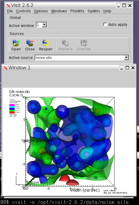
Contours of a scalar variable
- Open VisIt and
noise.silowith a single command or use File -> Openvisit -o /opt/visit-2.6.2/data/noise.silo
- Type
Ctrl+Ito display info about the data opened and then close the window - Click Add -> Contour -> hardyglobal
- Click Draw
- Double click on Contour (or Right-click ->Edit plot description)
- Under select by choose ->N Levels enter 5
- Change the opacity levels
- Click Apply
- Click Dismiss
- Click Delete
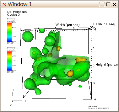
Pseudocolor and Isosurfaces for a scalar variable

- Click Add -> Pseudocolor -> hardyglobal
- Click Draw
- Click Operator -> Slicing -> Isosurface
- Click Draw
- Click Arrow to expand
- Double-Click Isosurface
- Under
Select bychoose ->Percent(s) enter 40 - Click Apply
- Rotate with a mouse
We will add additional isosurface at 80%
- Double-Click -> Pseudocolor
- Change Opacity
- Click Apply & Dismiss
- Click Add -> Pseudocolor -> hardyglobal
- Click Operator -> Slicing -> Isosurface
- Click Arrow to expand
- Double-Click Isosurface
- Disable
Apply operators to all plotson GUI window - Under
Select bychoose ->Percent(s) enter 80 - Click Apply -> Dismiss -> Draw

Clip Isosurfaces
- Click and enable -> apply operators and selection to all plots
- Click Operators -> Selection -> Clip
- Click Draw
- Double-Click -> Clip
- Click Plane 2
- Click Apply & Dismiss
- Click x (to delete)
- Click Draw

Slice Isosurfaces
Continue from previous example.
- Click Operators -> Slicing -> Slice
- Click Draw
- Double-Click -> Slice
- Click Z-Axis & Project to 2D
- Click Apply
- Click Dismiss

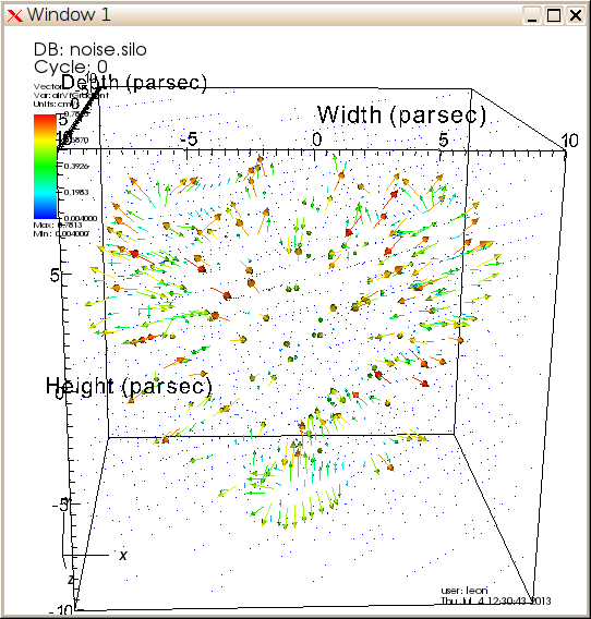
Create Glyph of Vector
- Unselect Apply operators/ selection to all plots
- Click Add -> Vector -> airVfGradient
- Click Draw
- Double click on Vector
- Under N vectors enter 4000
- Click Apply
- Click Dismiss
- Click
Hide/Showto hide.
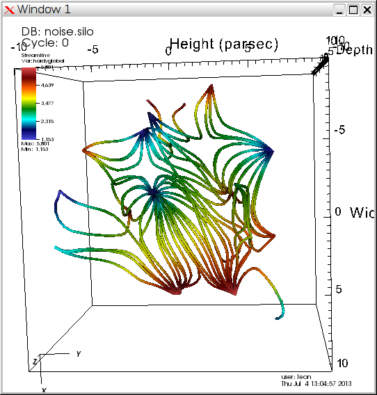
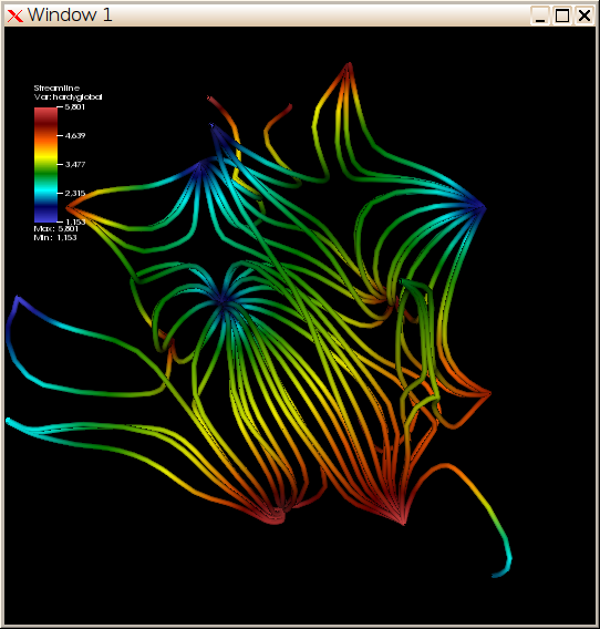
Create Streamlines

- Click Add -> Streamline -> grad
- Double click on Streamline
- Under Source Type Select Plane
- Enter:
- Samples in X: 8
- Samples in Y: 8
- Streamline Direction Both
- Click Apply
- Click Dismiss
- Click Draw
- Double click on Streamline
- Click on Appearance
- Under draw as select Tubes
- Click Apply
- Under Data Value select Variable
- Under Variable select Scalars -> hardyglobal
- Click Apply
- Under Color -> Color table, click Default Choose hot_desaturated
- Click Apply & Dismiss

Background Color and Legend
Continue from previous example.
- Click on Controls -> Annotation (Ctrl+N)
- Click on Colors
- Select Black for Background and White for Foreground
- Click Apply
- Click on General
- Click
No annotations - Click legend
- Click Apply & Dismiss
- Hide Pseudocolor Plots

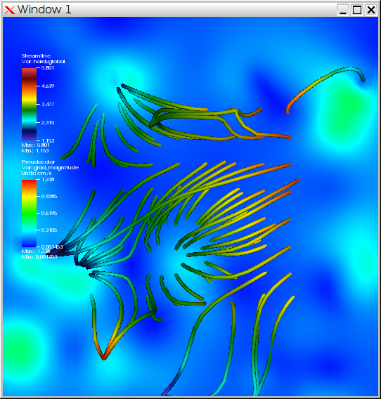
Create Slice
Continue from previous example.
- Click Add -> Pseudocolor -> grad_magnitude
- Click Draw
- Click Operator -> Slicing -> Slice
- Double click on Slice
- Select Z Axis
- Unselect project to 2D
- Click Apply & Dismiss
- Click Draw
- Click
Hide/Showon Streamline to show plots together - Hide everything
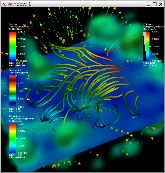
Create Volume Rendering
Continue from previous example.
- Click Add -> Volume -> grad_magnitude
- Click Draw (This might take some time but we continue anyway)
- Double click on Volume
- Change 1D Transfer Function graph by freely drawing in Opacity and removing lower range intensities.

- Click Apply
- Click Dismiss
- Show previous plots and explore results by rotating, zooming, switching ...


Attachments (11)
-
ex1.png (126.6 KB) - added by 13 years ago.
Contours of a scalar variable
-
ex2.png (89.7 KB) - added by 13 years ago.
Pseudocolor and Isosurfaces for a scalar variable
-
ex3.png (38.1 KB) - added by 13 years ago.
Clip Isosurfaces
-
ex4.png (13.2 KB) - added by 13 years ago.
Slice Isosurfaces
-
ex5.png (47.2 KB) - added by 13 years ago.
Create Glyph of Vector
-
ex6.png (92.2 KB) - added by 13 years ago.
Create Streamlines
-
ex7.png (137.0 KB) - added by 13 years ago.
Background Color and Legend
-
ex8.png (163.5 KB) - added by 13 years ago.
Create Slice
-
ex9.png (230.8 KB) - added by 13 years ago.
Create Volume Rendering
-
ex9-opacity.png (12.8 KB) - added by 13 years ago.
Opacity for volume rendering
-
noise.silo (10.7 MB) - added by 13 years ago.
Noise from VisIt examples
Download all attachments as: .zip